Interpolating thickness maps
With the Interpolate Map form, you specify the interpolation method that will be used to estimate the values at unknown points, by using the known data points. Optionally, to have more user control over the interpolation process, you can also add constraints or a trend map. As an alternative, you can use the property calculator to modify the thickness, see Modifying thickness values with the Property Calculator.
Select the thickness map you want to work with from the Thickness map drop-down list and continue further with the steps described per tab.
On the Interpolation tab, you have three options to select as the interpolation method: IDW (Inverse Distance Weighted), Kriging and Recursive Refinement.
To select an interpolation method
- Select the interpolation method from the Method drop-down list. The form will be populated with additional settings based on your selection.
- Fill in the settings for the selected method, see below for more information.
- Power The power parameter controls how strongly the weight depends on the distance from each data point. Any value greater than zero is allowed. Values between 0.5 and 10 are recommended. The default value of 2 produces a smooth interpolation and is appropriate for most applications. Smaller values for the power parameter generate more equal weights and interpolations approximating a constant value with spikes at each data point. Larger values for the power parameter generate larger weights for nearby data points and interpolations approximating a nearest neighbor interpolation.
- Advanced Settings (Only relevant when 'IDW', or 'Ordinary (legacy) Kriging' are selected under 'Method'.) Clicking the button opens the 'Advanced Settings' dialog. If you want to Apply trend analysis and data filtering, check the box at the top of the dialog. This will do the following:
- Optimize the computation time by allowing you to specify the number of data points used to calculate the output surface.
- The trend analysis, automatically carried out by the application, creates a relatively coarse regularly spaced grid in the specified area. The selected interpolation method is used to compute the values at these data points. A relatively fine spaced grid is then filled with the values from the coarse grid and adjusted with the local offset of the available data points. The filtering settings are then applied.
- Use <number> data points: Shows the total number of data points of the input object (for reference only).
- Use <number> trend analysis points: Shows the number of data points in the coarse, regularly spaced grid. You can edit this value, then click OK.
- When the number of input data points is less than 250, trend analysis is never applied.
- Trend analysis is automatically applied when the number of input data points is greater than: Kriging: 5000; Triangulation: 100000; Inverse Distance Weighting: 10000.
- Trend analysis is automatically applied when the number of output data points is greater than 100000.
JewelSuite Subsurface Modeling applies the following rules for trend analysis: - Type Select 'Ordinary', 'Ordinary (legacy)' or 'Simple':
- Ordinary The mean is unknown and only constant over the search ellipsoid. Good approach when there are many hard data and there is some evidence of non-stationarity. The industry standard Kriging library is used.
- Ordinary (legacy) This type of Ordinary Kriging does not make use of the industry standard Kriging library and is performance optimized. When you choose this option (as opposed to non-legacy Ordinary Kriging), the 'Advanced Settings' button at the base of the form becomes active and the 'Search Factor' is grayed-out.
- Simple The global mean is known and is held constant over the area of interpolation. Simple Kriging is the best approach when there is no or little evidence of significant non-stationarity and few hard data. The industry standard Kriging library is used.
- Variogram Type - Choose a variogram type to control how the variogram model is auto-fitted to the data:
- Exponential
- Exponential Power - Only available when 'Ordinary (legacy)' is selected under 'Type'. Set the value in the Power entry field, which sets the lateral extension of the kriging.
- Gaussian
- Spherical
- Major range - Specify the distance at which the values become independent (the variogram reaches its plateau). The distance is measured in the direction with the greatest spatial continuity. By default, the azimuth of the Major direction is 0°, and the azimuth of the Minor direction always perpendicular to it.
- Minor range - Specify the distance at which the values become independent (the variogram reaches its plateau). The distance is measured in the direction with the least spatial continuity and is orthogonal to the major direction.
- Azimuth (GN) - Enter the azimuth (angle with Northing direction) of the axis corresponding with the major range.
- Search factor - (Not available when 'Ordinary (legacy)' is selected under 'Type'.) The variogram model ranges are multiplied with the search factor to obtain the size of the search ellipsoid, i.e. Search ellipsoid = Search factor x Variogram model range. The search factor is applied to both ranges of the variogram model so that the shape of the search ellipsoid reflects the spatial anisotropy.
- Multiplier for initial coarse resolution - The number that is multiplied by the resolution of the specified area to produce the initial grid resolution. With the default value of 0, the method will automatically determine the most suitable multiplier value based on the desired final resolution and the distribution of your input data. Enter a number greater than the default in the entry field, or use the up and down arrows at the side of the field.
- Extrapolation method - Select an extrapolation method to ensure that the final map is fully populated with values (in cases of insufficient input data or input settings).
- None - Select this option to not extrapolate.
- Linear (default) - Extrapolate using a linear function.
- Quadratic - Extrapolate using a quadratic polynomial technique.
- Extrapolation area (active only when an extrapolation method is selected) - Specify the extent of the extrapolation by selecting one of the two options from the drop-down list:
- Outside convex hull - Extrapolate outside the convex hull around the input data.
- As needed (default) - Extrapolate in areas where grid nodes have not received a value.
- Grid nodes affected by snapping - The number of grid nodes that will be affected by each input data point. By default, the value of each input data point is assigned to the nearest 16 grid nodes. Enter a value less than the default value of 16 in the entry field, or use the up and down arrows at the side of the field.
- Click Apply to save the settings, interpolate the selected thickness map and keep the form open, or click OK to save the settings, interpolate the thickness map and close the form.
This method uses the inverse distance-weighted algorithm to interpolate the data. Inverse Distance Weighting (IDW) does not have a preference for direction and will only use the distance to data points as input for interpolating the surface. You can select the weighting exponent used for the weighting of the distances. In general the IDW method does not provide good results, as the algorithm is sensitive to the amount of input data. This means that especially added constraints will change the result drastically.
This method uses the Kriging algorithm to interpolate the data. The Kriging method also uses input locations as constraining input, but allows more options to be specified. You can select the variogram type, and specify the direction and range of the major and minor axis. The mean is unknown and only constant over the search ellipsoid.
Use this method to create maps with smooth contours, extrapolation and trends. The method creates a grid around your input data and assigns values from the data points to the nodes of the grid (snapping) in order to build the map. The grid starts with a coarse resolution and it is refined iteratively in order to reach the resolution of the area you specified on the Assign Data form. For more information on this interpolation method, see the section Recursive Refinement.
You can have more control over the interpolation process by adding user-defined thickness values as constraints.
You can adjust the display settings of the constraints, e.g. node size or font color, on the Display settings form (home > Settings > Display Settings > Objects > 2D Maps > Constraints).
- Visualize the map that you want add/edit constraints for in one of the following ways:
- Open the floating palette via clicking one of the following:
- Workspace > Tools > Editing Tools (Shift + F1)
- Open Editing Tools button
 on the Constraints tab on the Interpolate Map form
 - Select one of the tools depending on the type of constraint you want to create:
- Click on the map at the location(s) where you want to add a constraint.
- When you are done click on the Add Node
 tool, or the Extend Constraint
  tool to deactivate the tool.
 - The constraints are stored in the JewelExplorer under the selected map you are working with (Maps > Thickness Maps > Your Thickness Map > Constraints).
- A constraint entry is created on the Constraints tab on the Interpolate Map form. Type in a value in the table that will be used for that constraint (for a single node, or along a polyline or within the area of a patch). Every constraint can only have a single value.
- Click OK or Apply on the Interpolate Map form to interpolate the map using the constraint(s). All constraints that are checked on the form are used.
Open the map in a 2D View Thickness maps are stored in the JewelExplorer: Maps > Thickness Maps > Your Thickness Map > 2D Grid or Property.
Open the dedicated Thickness/Trend Map You can open the dedicated Thickness/Trend Map via opening one of the forms in the Thickness Maps workflows.
The editing tools for the constraints are distributed in two sections. The 'Create' section allows you to create new constraints. The 'Constraint Tools' section allows you to further edit your constraints such as by adding, moving or removing nodes.
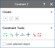
The editing tools for the constraints are distributed in two sections. click to enlarge

|
Create Node Constraint Create a constraint that consists of a single node. |

|
Create Polyline Constraint Create a constraint that consists of a polyline. |

|
Create Patch Constraint Create a patch constraint. |
When you select one of the tools the Add Node tool, or the Extend Constraint tool is activated.
For more information on working with the editing tools, see Graphically creating and editing constraints.
You have to use a boundary as a constraint in case you want to add user-defined thickness values in one of the following scenarios:
- Imported constraints When you have constraints that are created in another application, you first have to import them into JewelSuite using the data > Miscellaneous strip. Once you have imported the constraints, change the type to Boundary in the Inspector. It will be available in the drop-down list on the Add Constraints form.
- Constraints drawn in views other than the Thickness/Trend Map When you want to use a boundary as a constraint that was created in another view than the Thickness/Trend Map. You first have to create a new polyline set. Once you have created the polyline set, change the type of the polyline set to Boundary in the Inspector. It will be available in the drop-down list on the Add Constraints form.
- Existing boundary When you already have a boundary in your solution and you want to use it as a constraint.
- On the Interpolate Thickness Map form, select the Thickness map of interest in the Thickness map drop-down list on the form and for display in the JewelExplorer.
- Open the Add Constraints form with the Boundary Polyline Set button
 .
. - On the Add Constraints form select the boundary that you want to use as a constraint. For more information about boundaries, see Boundaries and Feature Sets.
- Click OK to add the selected boundary to the table on the Interpolate Thickness Map form.
- On the Interpolate Thickness Map form, type in a thickness for the constraint(s). Each constraint can only have one thickness.
- To apply the constraint(s) to the thickness map, click Apply to update the view and to inspect the results and keep the form open, or click OK to update the view and close the form.
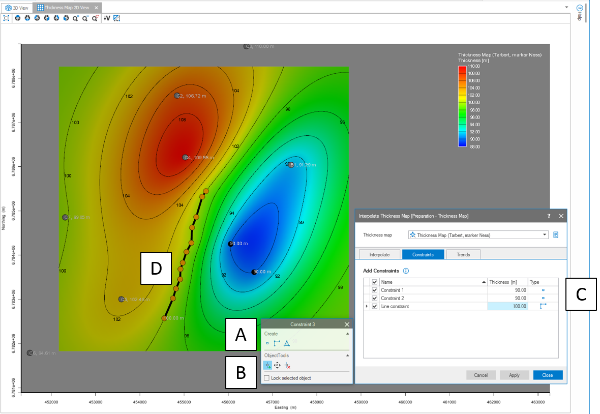
Adding constraints to a thickness map. When using the Constraints tab, you need to have access to the appropriate tools. In the Create section of the editing tools (A) you will find the icons to create new thickness constraints. The lower section (B) has the tools to add, move or remove constraint points. Upon creating a new constraint, it will be added to the table on the form (C), where you can enter a thickness value. Active constraints (D) are shown on the map with orange points. click to enlarge
On the Trends tab you can select a property to act as a trend. This trend property must be generated using the Property Calculator. Either you create an analytical trend based on a function, or project a thickness trend property from other objects into your thickness map area. If you want to use a trend, the property must to be based on the property type 'Thickness' to avoid unit conversion errors. Alternatively you can right-click on the thickness property of a thickness map and select Duplicate to create a copy and then modify name and values.
The trend has to be stored as a property under the thickness map to be available for selection on the form. Prior to interpolation, the trend is subtracted from the input data producing a thickness residual. This residual thickness is interpolated across the map. Then, the trend property is added back to this residual map to obtain the thickness map.
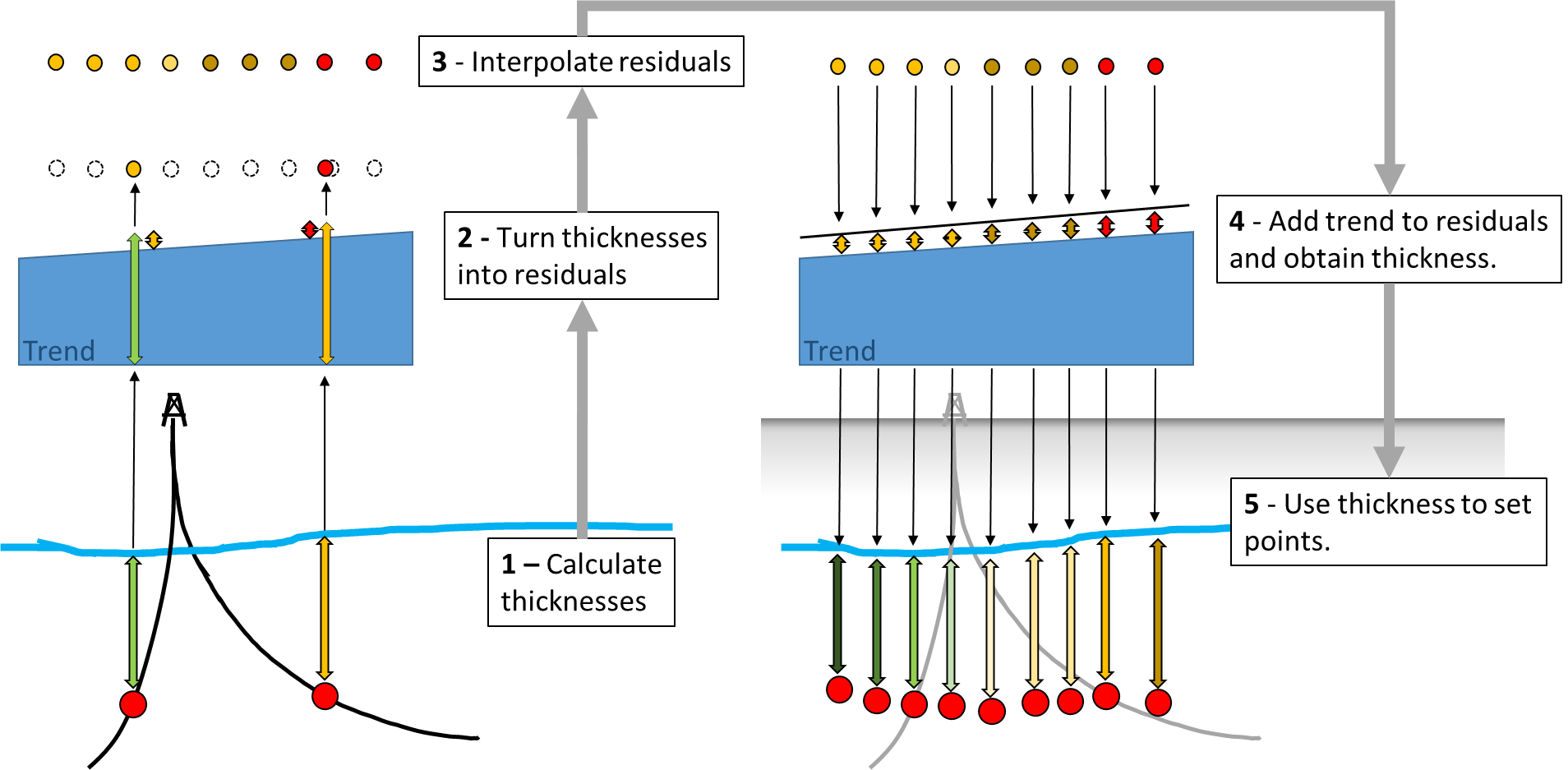
Working principle of a trend. (1) First the thickness values are calculated at the data locations. From these thicknesses, (2) the trend is subtracted which will generate residual thicknesses. (3) The residuals are then interpolated across the specified area according to the interpolation settings. (4) To obtain thicknesses again, the residuals are added to the trend. This map is then exposed to the user. (5) The final map can then be applied to a reference surface. click to enlarge
To add a trend
- Select the Thickness map of interest both in the Thickness map drop-down list on the form and for display in the JewelExplorer.
- Select a trend property from the drop-down list.
- To apply the trend to the thickness map, click Apply to update the view and to inspect the results and keep the form open, or click OK to update the view and close the form.
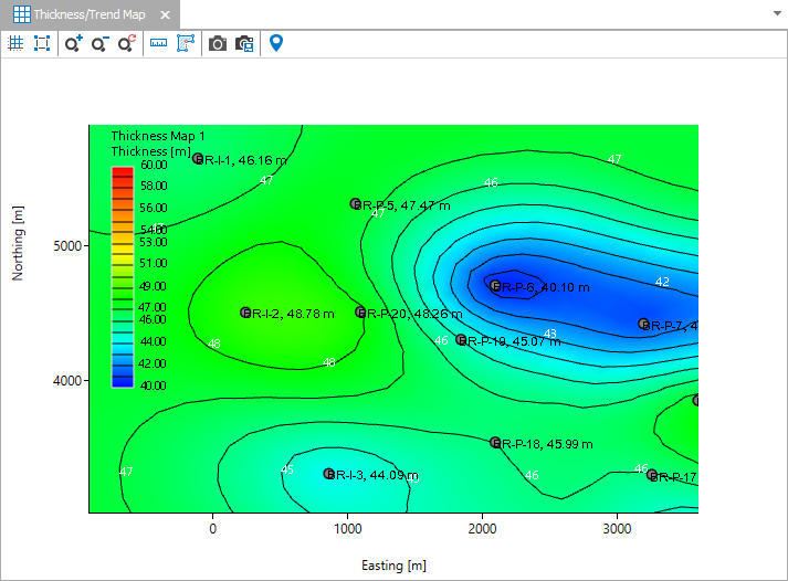
Example of a thickness map interpolation result. click to enlarge
The interpolated thickness map is available as a property with the name Thickness under the thickness map in the JewelExplorer.
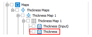
After completing this step, a thickness property will appear in the JewelExplorer under the thickness map. click to enlarge